Embedded Systems and Power Electronics

Total Pageviews

About Me

My photo
I am currently a PhD student at UC Berkeley, following a 6-year journey working at Apple after my undergrad years at Cornell University. I am a 2025 Paul & Daisy Soros fellow. I grew up in Dhaka, Bangladesh where my interest in electronics was cultivated, resulting in the creation of this blog.

BTemplates.com

Powered by Blogger.

Aug 5, 2025

Why is my buck output ripple higher than expected: ceramic capacitor derating vs voltage


Fig. 0a - The test hardware comprising a buck converter operating at 50kHz and 50% duty cycle. The PWM signals are generated from an on-board RP2040. The buck inductor (not shown) is soldered on the reverse side of the PCB.
Fig. 0b - Back side of the test PCB, where the input electrolytic caps and output inductor are soldered.


Fig. 1 - Buck converter

In a typical buck converter shown in Fig. 1, the output ripple voltage is an important design specification. Sensitive loads may specify a maximum ripple voltage. The max allowable voltage for the load is also limited by the ripple, especially for loads with tight specifications such as many processors.

The output ripple voltage is given by

\[ \Delta V_\mathrm{out} = \frac{V_\mathrm{in}D(1-D)}{8LCf_\mathrm{sw}^2} \]

The derivation is given at the end of this post for those interested. The different parameters are:

  • \( \Delta V_\mathrm{out} \) = peak-to-peak output ripple voltage
  • \( V_\mathrm{in} \) = input voltage
  • \( D \) = duty cycle
  • \( L \) = inductance
  • \( C \) = output capacitance
  • \( f_\mathrm{sw} \) = switching frequency

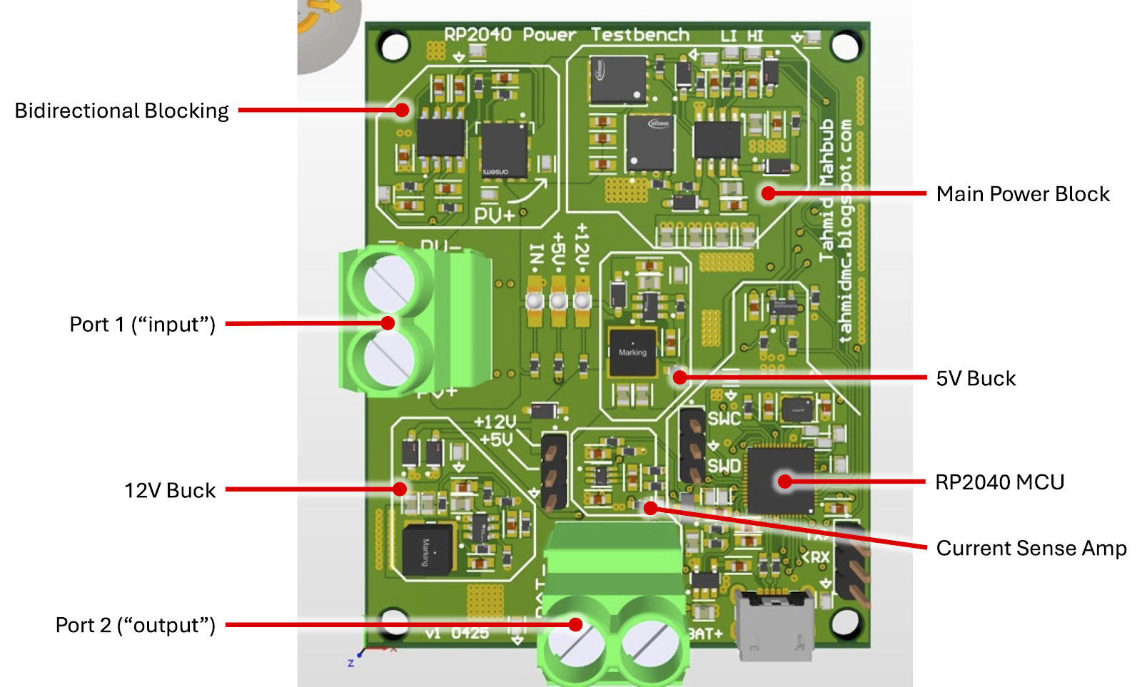
We can look at the output ripple using the power testbench. The converter is run at 50kHz and 50% duty cycle, with varying input voltages. The output capacitor of the converter is the parallel combination of 4x 0805 10µF caps (GRM21BR61H106KE43) and 1x 1206 10µF cap (CGA5L3X5R1H106K160AB). The inductor is rated at 5.6µH, specifically the Wurth 732-3799-1-ND.

Based on this, you would expect the output ripple at 10V input to be given by:

\[ \Delta V_\mathrm{out} = \frac{V_\mathrm{in}D(1-D)}{8LCf_\mathrm{sw}^2} = \frac{10V \cdot 0.5 \cdot 0.5}{8\cdot 5.6\mu H \cdot 50\mu F \cdot (50\;kHz)^2} =0.45\;V \]

The ripple waveform is obtained with a scope that is AC coupled and can be seen below in Fig. 2. From the scope shot, it appears that the voltage ripple is about 0.75V, which is a fair bit higher than the expected ripple. So what gives?

Fig. 2 - Output ripple, AC coupled, 500mV/division, Vin=10V, Vout=5V

The culprit here is voltage derating of ceramic capacitors. Much like how I've previously written about electrolytic capacitors derating with frequency, ceramic capacitors (particularly class II dielectrics) can derate substantially with voltage. This has to do with the reduced permittivity of the dielectric, reducing the capacitors' ability to store energy at higher voltage biases. This is often given in manufacturer technical documentation. For our caps, the derating charts are reproduced below.

Fig. 3a - GRM21BR61H106KE43 DC bias characteristics, credit: Murata

Fig. 3b - GRM21BR61H106KE43 5V DC bias corresponds to a 6.4µF capacitance

Fig. 4a - CGA5L3X5R1H106K160AB DC bias characteristics, credit: TDK

Fig. 4b - CGA5L3X5R1H106K160AB 5V DC bias corresponds to a 9.1µF capacitance; you will often notice that larger packages correspond to reduced derating and hence have larger capacitances for the same initial capacitance and voltage rating

Considering the derating from Figs. 3-4, the total output capacitance is 34µF. With this new value plugged in, the expected output ripple is about 

\[ \Delta V_\mathrm{out} = \frac{V_\mathrm{in}D(1-D)}{8LCf_\mathrm{sw}^2} = \frac{10V \cdot 0.5 \cdot 0.5}{8\cdot 5.6\mu H \cdot 34.7\mu F \cdot (50\;kHz)^2} =0.64\;V \]

This is much closer to the observed value with a 14.5% error, something that is fairly within the tolerance of different components.

If we now look at the results with 20V input (corresponding to 10V output), we would expect an output ripple of double that for the 10V input, corresponding to 1.3V; if the caps didn't further derate. However, we can find again from the manufacturer data that the total output capacitance is 19.7µF, down from 34µF, which would correspond to a greater increase in the ripple. This is shown in Figs. 5a and 5b.

Fig. 5a - GRM21BR61H106KE43 10V DC bias corresponds to a 3.2µF capacitance

Fig. 5b - CGA5L3X5R1H106K160AB 10V DC bias corresponds to a 6.9µF capacitance

Fig. 6 - Output ripple, AC coupled, 500mV/division, Vin=20V, Vout=10V

The output ripple observed with 20V input is shown in Fig. 6. The measured ripple corresponds to 2.7V, which further highlights the substantial capacitance drop with 10V bias for the output ceramic capacitors!

The expected ripple with ideal caps is given by
\[ \Delta V_\mathrm{out} = \frac{V_\mathrm{in}D(1-D)}{8LCf_\mathrm{sw}^2} = \frac{20V \cdot 0.5 \cdot 0.5}{8\cdot 5.6\mu H \cdot 50\mu F \cdot (50\;kHz)^2} = 0.9\;V \]

However, with derated capacitance, the expected ripple is 

\[ \Delta V_\mathrm{out} = \frac{V_\mathrm{in}D(1-D)}{8LCf_\mathrm{sw}^2} = \frac{20V \cdot 0.5 \cdot 0.5}{8\cdot 5.6\mu H \cdot 19.7\mu F \cdot (50\;kHz)^2} = 2.3\;V \]
This is much closer to the observed ripple value.

For proper filtering, it is crucial to consider the DC bias impact on the ceramic capacitors and the corresponding derating, in addition to component tolerance! Otherwise, the filtering will be insufficient and the ripple will be much higher than expected, as shown here. This could result in poor circuit performance or even component damage!

Note that the circuit parameters here were chosen to have large output ripple to illustrate the concern described in this article. In almost any application, this circuit has a very high ripple percentage. Even with the components as present, the frequency can be increased substantially to reduce the ripple. Alternately, the output inductor or capacitance can be increased.

Ripple Derivation

Fig. D1 - Buck Converter


Fig. D2 - Buck Converter when QH is on


Fig. D3 - Buck Converter when QL is on

To find the output ripple in a buck converter, we start from the inductor current, which can be determined from the inductor voltage in either QH on or QL on state. We can identify that \( i_\mathrm{L} \) increases when QH is on since \( v_\mathrm{L} \) is positive then. And similarly, \( i_\mathrm{L} \) decreases when QL is on since \( v_\mathrm{L} \) is negative.

QH is on for a fraction of the switching period given by the duty cycle D. For a buck converter, the output voltage is given by \( V_\mathrm{out} = D V_\mathrm{in} \). The inductor voltage relationship \( v_\mathrm{L} = L \frac{di_\mathrm{L}}{dt} \) can be rewritten for constant voltage \( v_\mathrm{L} = L \frac{\Delta i_\mathrm{L}}{\Delta t} = L \frac{\Delta i_\mathrm{L}}{D T_\mathrm{sw}} \) where \(T_\mathrm{sw}\) is the switching period.

The peak-to-peak inductor current ripple is thus given by
\[ \Delta i_\mathrm{L,pp} =  \frac{V_\mathrm{in}-V_\mathrm{out}}{L}\cdot \frac{D}{f_\mathrm{sw}} = \frac{V_\mathrm{in}(1-D)D}{Lf_\mathrm{sw}} \]
We know from Fig. D1 that \( i_\mathrm{L} = i_\mathrm{C} + i_\mathrm{out} \). We can find the impedance of the output capacitor and determine the current split between it and the output load. We can assume (and confirm mathematically) that the impedance of the output cap at high frequencies (such as in a typical buck converter) is much lower than the load resistance. Thus, we can assume that the inductor ripple current is going through the output cap, as shown in Fig. D4, and that the DC amount is going through the load resistor.
Fig. D4 - Current going through the output capacitor

When the ripple current is positive (for half of \( T_\mathrm{sw} \) ), the output capacitor is charged and when the ripple current is negative, the output capacitor is discharged. The peak-to-peak capacitor voltage ripple can be found from the positive inductor current charging the cap, where Q is the charge \( \int i_\mathrm{C}\;dt = \frac{1}{2} \frac{\Delta i_\mathrm{L,pp}}{2} \frac{T_\mathrm{sw}}{2} = \frac{1}{8} \Delta \frac{i_\mathrm{L,pp}}{f_\mathrm{sw}} \)

\[  \Delta V_\mathrm{out} = \frac{Q}{C} = \frac{1}{8Cf_\mathrm{sw}} \Delta {i_\mathrm{L,pp}} = \frac{1}{8Cf_\mathrm{sw}} \frac{V_\mathrm{in}(1-D)D}{Lf_\mathrm{sw}} = \boxed{ \frac{V_\mathrm{in}D(1-D)}{8LCf_\mathrm{sw}^2} } \]

As a final check, we can go back to checking the magnitude of the output capacitance compared to the load resistance (10Ω output resistor was used) with the circuit in Fig. 0.
\[ |Z_\mathrm{C}| = \frac{1}{2 \pi f_\mathrm{sw} C} = \frac{1}{2 \pi 50\;kHz \; 19.7\mu F} = 0.16 \Omega \ll 10 \Omega \] 

May 1, 2025

Using a PV panel indoors by biasing with an external power supply


My introduction to working with solar panels goes back a long time. In fact, in 2012, I posted this article when I was working on some charge controllers and inverters. One consistent challenge when doing such work is always having a consistent reliable PV panel outdoors in bright (ideally not-too-hot) sunlight. This becomes difficult with varying weather conditions and limits development.

Recently I learned about how you can very easily use an external power supply (capable of operating in constant current mode) to use the PV panel indoors and emulate its outdoor behavior! This ends up being great for testing charge controllers and MPPT algorithms!

Fig. 1 - Setup for characterizing PV panel behavior indoors
Panel: SLP010-12U
Power supply: Rigol DP832
Eload: Rigol DL3031

Fig. 1 shows the test setup used for obtaining PV panel IV curves indoors. The only equipment required for emulating the PV panel itself is the power supply. The electronic load is used to vary the voltage imposed on the panel to obtain the IV curve. You can even see the panel facing down so that light is not incident onto it!

Fig. 2 - Simple PV panel model

We can start by recognizing that a PV panel may be simply modeled as shown in Fig. 2. Iph represents the photocurrent generated by the panel under sunlight. When the panel is indoors, Iph is a miniscule value under typical indoor lighting conditions. What we can do is, instead, use an external power supply to bias the panel with a constant current source. This is represented by Iext in Fig. 3. 

Fig. 3 - External power supply used to emulate photocurrent in PV panel

This is as simple as configuring the power supply's voltage at (or higher than) the panel's open-circuit voltage (Voc), and setting the current limit at the panel's short-circuit current (Isc). For the panel I picked, these correspond to 21.6V and 0.68A (at 100% luminosity).

The short-circuit current limit for the PSU can be varied to provide Iext emulating varying luminosities! For example, using 50% of the panel's short-circuit current, a condition of approximately 50% luminosity may be emulated!

This may be taken even further by adding a series voltage source to emulate voltage shifts in the IV curve.

Tests with 10W panel:

To generate the IV curves in a repeatable fashion, I wrote a Python script that imposes different panel voltages by issuing the corresponding SCPI commands to the electronic load. The curve is then plotted in real-time, as shown in Vid. 1 below. The GUI was built by modifying the one from a previous blog post: SmartSinePy, and an example of GUI development with PySide6 ~ Tahmid's blog

Vid. 1 - Characterizing panel IV curve at 100% emulated luminosity

To illustrate the operation at 50% emulated luminosity, the power supply current is set to 0.34A instead of 0.68A. The corresponding curve is generated as shown in Vid. 2.

Vid. 2 - Characterizing panel IV curve at 50% emulated luminosity

These obtained curves are also shown below in Fig. 4 and Fig. 5.
Fig. 4 - Obtained IV curve at 100% emulated luminosity

Fig. 5 - Obtained IV curves at 100% (top, same as Fig. 4) and 50% (bottom) emulated luminosities

Fig. 6 - IV curves provided in the panel datasheet

Fig. 6 shows the IV curves of the panel from its datasheet, showing close agreement between the curves obtained indoors with the 25°C curve! Slight tweaking of the open-circuit voltage and short-circuit current to match the 25°C curve can give slightly better match!

More significantly, this now allows testing with the PV panel indoors without worrying about weather conditions! Of course, all final tests for any charge controller or MPPT algorithm should be run outdoors with the panel under varying weather conditions, but this emulation method can significantly improve development time. I will soon share a demonstration of an MPPT controller developed using this setup!

Characterization of a 100W panel:

The same technique can be used for different panels and power levels. Fig. 6 shows one such IV curve obtained using the techniques outlined here but with a more capable power supply and electronic load. The power supply was set to 24.3V (panel open-circuit voltage) and 5.21A (panel short-circuit current at 100% luminosity).
Fig. 6 - Obtained IV curve for a 100W panel

This simple technique can significantly improve development and testing times for projects using PV panels! For more details about this emulation technique and further enhancements, refer to the following papers which provide much greater detail:

1. S. Qin, K. A. Kim and R. C. N. Pilawa-Podgurski, "Laboratory emulation of a photovoltaic module for controllable insolation and realistic dynamic performance," 2013 IEEE Power and Energy Conference at Illinois (PECI), Urbana, IL, USA, 2013, pp. 23-29, doi: 10.1109/PECI.2013.6506029.
https://ieeexplore.ieee.org/stamp/stamp.jsp?tp=&arnumber=6506029

2. T. -L. Huang, F. S. Bagci and K. A. Kim, "Indoor Panel-Based Photovoltaic Emulation Method Implementation and Evaluation," 2024 IEEE Workshop on Control and Modeling for Power Electronics (COMPEL), Lahore, Pakistan, 2024, pp. 1-7, doi: 10.1109/COMPEL57542.2024.10613957.
https://ieeexplore.ieee.org/stamp/stamp.jsp?tp=&arnumber=10613957

Mar 30, 2025

Power Testbench and Upcoming Power Electronics Tutorials


While I have written many articles on this blog about power electronics related topics, I am hoping to share more fundamentally structured tutorials and articles, based on power electronics fundamentals that have been reinforced during my time in graduate school. To that end, I have designed a testbench to cover topics ranging from basics to slightly more involved ones. I have completed the design of a power electronics test bench, sent out the PCB files to be fabbed at OSHPark, and ordered parts from Digikey.

Here are some ideas I have for topics to cover, and I'd love to get feedback on other topics of interest!

Here are a couple 3D renders of the testbench hardware from Altium:

Top side render

Bottom side render

I will go over more details of the design and will be sharing the Altium design files and bringup progress when the board is back! I am hoping to use this design and framework to provide more structured tutorials on power electronics, building on past articles on this blog.

Jan 1, 2025

Sprucing up an old scope: fixing the dials on the Owon SDS6062V


I got the Owon SDS6062V scope back in 2014 when it seemed a great deal compared to brands like Tektronix and much better than cheaper analog or portable digital scopes. These days, I've been using the Rigol DS1202 for hobby projects which is a better part, in my opinion. Of course, none of these are as nice as the Keysight MSOX scopes at work.

I've demonstrated the Owon scope in previous projects such as Generating complementary PWM with adjustable deadtime for the RP2040 and Stereo audio player using the PIC32, MCP4822, microSD card and the MDDFS library (back in 2015!). The dials on the front panel seem to all be "broken". When turning the dials, the response is erratic. For example, when turning the time division dial clockwise, sometimes the time division goes up, sometimes down, sometimes it jumps all the way down to the minimum or will jump up and back down. The same is true for all the other dials. Searching online revealed that this seems to be a common issue with the scope, with the encoders having worn out with age. Some sources suggested using filter caps on the output of the encoders (dials). However, this didn't help with mine. So I decided to just replace the encoders themselves.

The instructions for taking the scope apart and getting to the front panel PCB that houses the encoders is very well documented in the service manual. I uploaded a copy of the Owon service manual on Drive: Owon Service Manual (Drive mirror)


Fig. 1 - Owon SDS-6062V oscilloscope with original dials and caps

Fig. 2 - Scope with the encoders replaced

Fig. 3 - The front panel PCB with the encoders soldered

After accessing the front panel PCB, I desoldered all the encoders. I could not find part numbers for these encoders and just went ahead and bought a standard 10-pack of encoders (Amazon link). Fig. 4 shows that the ordered parts are quite a bit taller than the ones on the scope. However, with the different encoder caps as shown in Fig. 5, the height difference is substantially removed. When I was looking online for which encoders to order, I found several sources suggesting ordering "standard encoders" without part numbers. So my hope here is that if someone is trying to change the encoders on their scope, they have a reference part to order if they're lost.
Fig. 4 - Encoders for the scope. Left = encoders removed from the scope PCB. Right = encoders ordered from Amazon.

Fig. 5 - Encoders with their corresponding caps mounted. Left = encoders removed from the scope PCB. Right = encoders ordered from Amazon.

Once the new encoders are soldered into the panel, the scope dials now worked as expected. The replacement encoders I used all have steps in them. The scope's horizontal position encoders did not have steps. I didn't mind this at all and actually quite like the additional tactile feedback.

I am also a big fan of the look of the new encoder caps! The spruced up scope is shown in Fig. 2. This was a simple fix, but I wanted to document the service manual and the encoders here for someone else to find useful! This breathes new life into this trusty scope and hopefully it can continue functioning!

Here are some fun shots of the interior of the scope!


Dec 31, 2024

Insights from repairing a 30V 5A power supply (BPS-305)


When I started working on a project (hopefully more on that soon), I reached out for an old 30V 5A power supply (Lavolta BPS-305). I rotated the voltage dial to try to get to 24V and observed that the voltage would not go past 15V, even though it is rated for 30V. Even though this supply was a few years old, I had not personally used it before. So, it wasn't clear whether it was a previously-functioning supply that stopped working, or whether it was always broken.

Fig. 1 - Lavolta BPS-305 power supply

Upon some more poking and prodding, I identified that the power supply had several issues:

  1. Output voltage only goes up to about 15V instead of 30V max.
  2. Output voltage is not stable and fluctuates at steady state, appearing unregulated. See video below.
  3. Output voltage flickers when relays switch around ~7V and ~14V and the relays keep flickering unless the voltage is moved far away from the transition points.
  4. Output current measurement (when HI/LO button is pressed down to LO) is off by a factor of 2.
  5. Output current measurement (when HI/LO button is pressed up to HI) displays zero.
Output voltage unstable at "steady state" - moving between 10.2V to 11.1V with a fixed output load

Hopeful that I can repair the supply, I opened it up. Noticing a relatively simple one-layer PCB, I set out to find a schematic or other reference for the supply. This is where I realized that many many (low-cost) 30V 5A power supplies are based on the same couple designs. I'll link to a few useful resources here that I came across during my search:

Instead of going through all my investigations, I'll highlight a few standouts here.

Broken potentiometers

After lots of investigating, the key offenders were 2 broken potentiometers. Referring to the file PS305D Schematic Main in the Drive link, these are VR104 and VR102. These are shown below in Fig. 2.
Fig. 2 - The culprits. VR104 is marked 502 (5kΩ) and VR102 is marked 501 (500Ω). Both parts measure open at component ends.

VR104 is used for output voltage feedback. Once this part was replaced with a functioning 5kΩ pot, the output voltage was now stable and would go all the way up to 30V. The pot is trimmed until the max output voltage is 30V.

VR102 sets the max output current when the HI/LO button is released (HI -> 5A current limit). There was no current limit being set in this setting with the faulty part. Since I did not have a 500Ω pot on hand, I replaced VR102 with a 5kΩ pot in parallel with a 470Ω resistor. This allows tuning the resistance as shown in Fig. 3. Fig. 4 shows the parallel 470Ω resistor soldered on the back side of the board. Once these parts were provisioned, the 5kΩ pot was trimmed until the max output current was set to 5A. The red dot in Fig. 3 indicates the final trimmed resistance.

Fig. 3 - combined resistance of 5kΩ pot in parallel with 470Ω resistance as the pot is trimmed.

Fig. 4 - soldered 470Ω resistor in parallel with VR102

FIg. 5 - the two blue potentiometers replace the broken ones in Fig. 2

Tuning the current display

Fig. 6 - Output current reading 6.89A when the real measured value is 5A
Fig. 7 - DMM on the PSU; the trim pots are the blue components near each chip. Left display is for current and the corresponding trimpot is VR211. Right display is for voltage and the corresponding trimpot is VR201.

When the HI/LO button is pushed down to the LO position, the PSU's output current limit is set to 2.5A tuned by VR101. When the HI/LO button is at the HI position, the output limit is set by VR102 (and the parallel 470Ω resistor) as described previously. However, there was a fair bit of error on this reading, as shown in Fig. 6. By adjusting VR305 (see PS305D Schematic Controls in the Drive link) in conjunction with the reference voltage set by the blue trimpot VR211 (see PS305D Schematic Display in the Drive link) in Fig. 7, the output current can be tuned. Since VR211 affects the reference voltage for the current meter, adjusting it affects both the HI and LO current readings. The procedure then was to set the switch to HI and then tune VR211; once that is corrected, switch to LO and then tune VR305.

Relay-selectable transformer secondary winding

Fig. 8 - secondary selection scheme with relay

Because the regulation stage in the power supply is based on a linear regulator, the difference between the input and output power is dissipated as heat. Since the power supply has a large selectable output range, this would result in very high power dissipation in the regulator at lower input voltages. To overcome this drawback and reduce the power dissipation, the power supply utilizes a selector circuit on the secondary as shown in Fig. 8.

As an example, let's consider that the output power is desired to be 3.3V. Suppose the input voltage post-rectifier is 40V (which is the case between S3-S0 for the BPS-305). At an output current of 3A, the power dissipated in the regulator would be roughly: Pout-Pin = Vout*Iout - Vin*Iin ~ (Vout-Vin)*Iout = 110.1W.  All this for only 13.2W of output power. At lower output voltages and higher output currents, this gets even worse!

By using the scheme shown in Fig. 8, the voltage at the input of the regulator is selected based on the desired output voltage to reduce power dissipation. With the example above, now suppose that for 3.3V, the input to the regulator is 14.8V, the power dissipation is reduced to 34.5W now! That's 75W less than the previous example!

For my unit, the voltage bins transitions happen for output voltages 8V, 15V, 21V and 30V. This is a good design decision rather than having a fixed 40V input for the regulator.

Output testing

For testing the output, different resistor combinations were used as the load. In addition, a constant current circuit was used even as the output voltage is varied. A simple circuit can be designed using the jellybean LM317 part. The datasheet shows an example circuit in Section 9.3.3 (Precision Current-Limiter Circuit).
Fig. 9 - constant current circuit using LM317

The output (ADJUST pin) is tied to GND for testing. Using R1 = 4.7Ω provides a ~250mA constant current load. Similarly, R1 is swapped out for lower values for higher currents. It is important to have a heatsink mounted on the LM317, especially at higher voltages. This constant current value was also used to validate the output current display across PSU output voltages.

Other observations

  1. The logic GND for the electronics are shorted to the positive output instead of the negative output. Even though the circuits in the PSU closely reflect those of PS305D Schematic Main/Display/Controls, this grounding scheme is reflected in hy_3005_dc_power_supply.
  2. Many of these 30V 5A power supplies seem to be based on a couple base designs with slight tweaks in implementation.
  3. The build quality appears shoddy. Many components were haphazardly soldered - many caps weren't fully seated. The fan wires run adjacent to (and touch) the (potentially very hot) heatsink for the transistors. However, none of these appear to impact functionality, at least in the short term.

Jul 10, 2024

A low-cost high-side current sense amplifier: design considering non-idealities


Current-sensing is commonly used in power electronics and embedded systems, both for system monitoring, as well as to take decisions. Examples of common use cases for the latter are:
  1. Monitoring inductor current for current-mode control in power converters
  2. Monitoring converter current for overcurrent protection
  3. Reading battery charge current to inform the charging process
  4. Reading output current to compute output power to inform how to proceed in an MPPT charge controller
Use cases 1 and 2 require high-speed current measurements since they need to operate at either the converter's control frequency or based on a desired response time. Use cases 3 and 4, however, only require measuring "DC" current and so don't require high-speed current sense. The high-speed aspect ties to notions of slew rate and bandwidth for the amplifier. Other non-idealities, which I will describe here, affect even the DC behavior of the amplifier.

High-Side vs Low-Side Current Sensing

This article gives a good overview of the differences between high-side and low-side current sensing. Shown below are what they look like.

(a): High-side current sense
(b): Low-side current sense

Sense Resistor Selection

In both cases, the sense element is the series resistor Rs. By monitoring the voltage drop across Rs, you can compute the corresponding current from Ohm's Law: V=IR.

Tradeoffs for resistor selection include considerations for power and minimum sense voltage.
  • Power dissipation in the resistor is given by Irms2Rs. A larger resistor will correspond to larger power dissipation for the same current.
  • Using a small resistor corresponds to a smaller sense voltage. When using a small sense resistor, you will use a current sense amplifier (CSA) to amplify the small sensed voltage to feed the corresponding circuit, which is often an ADC. A smaller resistor will correspond to requiring a larger gain in the amplifier or a greater ADC resolution.

High-side vs low-side

High-side current sense refers to placing the sense resistor in the "power" side without disrupting the power return or ground, enabling  the use of a common ground overall circuit scheme. Low-side current sense refers to placing the sense resistor in the "ground" side, thereby disrupting the power return/ground. If common-ground is not desired for your application, you can use the low-side sense scheme. 

In this article, we're looking at applications where you prefer high-side current sense!

Non-idealities Considerations and Circuit Design

In this application, I'm focusing on using a standard ultra-cheap op-amp instead of a dedicated current sense amplifier (such as INA180).

The op-amp I'm picking for this is the TL082 which I have on hand. The amplifier design is based on a standard differential amplifier configuration as shown in this article. The datasheet for the TL082 can be found on the TI website [1] [2]. LCSC shows the ultra-low cost of < $0.20 at volume!

The schematic for the current-sense amplifier (CSA) is shown below.

CSA implementation circuit (click to enlarge schematic)
R1=R2=2.2kΩ, R3=R4=5.6kΩ, Rs=0.5Ω, C1=C2=4.7uF, C3=0.1uF
VSNS+ = 12V


There are 3 parts to the output to consider:
  1. VREF biases the output to 5V. Errors in the 5V reference will propagate to the output.
  2. The diffamp gain is given by R3/R1 assuming R1=R2 and R3=R4. The input to the diffamp is given by the voltage across the sense resistor, which is the product of the current through it and its resistance.
  3. The slope of the output voltage against current is negative due to the diffamp having negative gain. This is by design. See below.

We need to consider the amplifier non-idealities when designing the part. The ones we are considering, along with their impacts is shown below.

  1. Input offset voltage
    • This is a mismatch in the input voltage of the op-amp, due to the input-side design of the op-amp itself. This gets amplified and shows up as an error on the output. The TL082 is specced at 5mV typically. With our amplifier's gain of 5.6/2.2=2.54, this means that this offset shows up at the output as ~12.7mV. Given that our system's current gain magnitude is 1.27V/A, this corresponds to a 10mA error in current reading.
    • Note that the offset can be positive or negative.
    • Additionally, the offset varies over part tolerances and temperature, going up to as much as 20mV, which will correspond to closer to 40mA of error.
    • Whether this is a problem or not depends on your application and desired current sense accuracy. You can perform an offset calibration to try to get rid of the steady-state error and only have to worry about the smaller temperature-dependent offset error. Alternately, you can use an opamp such as the TL081 which has additional pins to allow for offset nulling.
    • Better opamps with lower offset can be used if the offset is an issue and cannot be solved by calibration.
  2. Input bias and offset current
    • A large input bias current will correspond to voltages dropped across R1 and R2, which will correspond to errors in the sensed voltage. The TL082 has bias currents in the 50pA-8nA range. Since this shows up on both inputs on this amplifier, the impact will depend on the mismatch between the input resistors. This will not be an issue in this particular application. In a low-side current-sense amplifier, the bias will show up differentially since one side will likely be grounded, so you will need to be more careful there.
    • A large input offset current will correspond to mismatch in this voltage dropped across the input resistors, which will get amplified and show up as an error on the output. The TL082 has an input offset current spec between 25pA-4nA. The impact of this is the same as for the input offset voltage. Given that the input offset voltage spec is worse than this corresponding offset, this can be ignored for this application.
    • The design will tend to get more sensitive to bias/offset current if you use larger input resistors, so you should be careful about that.
  3. Input common-mode voltage range
    • Rail-to-rail opamps allow the input voltages to go as high as the supply voltage and as low as the supply return. However, the TL082 is not a rail-to-rail opamp, so you need to be careful about making sure that the input voltage is within the desired spec. The datasheet outlines that the input voltage can go as high as the supply rail but can only go as low as 4V above supply return. That means that in our single-rail application, the input voltage cannot go below 4V.
    • Note that this limit also means that you should not use the TL082 to buffer voltages below 4V!
    • With the 5.6k and 2.2k resistors, as well as the 5V VREF, this is not a concern in our application! However, this is something to keep in mind!
  4. Output voltage range
    • You can notice that I flipped the + and - inputs on the op-amp relative to a non-inverting configuration. This gives negative gain, but why did I do this? By using VREF=5V, this then means that as current goes up, the output voltage will go down but will nominally be 5V. If I used VREF=0V and used a non-inverting configuration, that would result in the desired 0A output to be 0V. However, the TL082 cannot drive its output to within 200mV of the supply rail or return (or even worse if you have too low an output resistance!).
    • This means that if the output sits at 200mV with no input, we cannot resolve currents below 158mA. However, if we sit at 5V, we don't have this issue since 5V is far out from either supply rail or GND!
    • With a large enough current, the output still can't swing low enough, so the max current we can resolve is about (5V-0.2V)/1.27[V/A]=3.8A. Note that this would result in a large power in the sense resistor, so this is another constraint to consider!

Some additional considerations:
  • VSNS+ is bounded between 4V and 14.75V. The lower bound maintains the op-amp's input common mode voltage range. The upper bound is given by the op-amp's supply voltage (=12V here). VSNS+ can go higher than 12V as long as the input to the op-amp pins is maintained to be at most 12V. The op-amp voltage at its non-inverting input is given by the equation below. With the circuit components implemented, this sets the upper bound of VSNS+ to 14.75V.

  • Errors in the reference voltage VREF (=5V here) will propagate to the output. These can be accounted for with an initial calibration step. For best performance, use a voltage ref chip such as the LM4040. This will give better accuracy for the voltage reference.
  • You can set the VREF to a higher voltage and increase the gain.
  • You can use a voltage divider at the output to rescale the output to a lower range.
  • You should add a low-pass anti-aliasing filter between the current-sense amplifier's output and the next-stage ADC.

Measurements

With steady state currents, the following output voltages were measured.
  • 0.33A : 4.70V measured vs 4.58V expected : +2.6% error
  • 0.94A : 3.73V measured vs 3.81V expected : -2.0% error

The input offset contributes output error - with no input, you can measure the output and find the offset. The component tolerances also contribute additional error.

For the purposes of this demonstrative application, this is deemed sufficient! In a wide range of applications, this could also be sufficient, especially in cases where the application is very cost-sensitive! I wanted to share some of the non-ideality considerations through this application and would love to hear if this has helped you understand them!